Architecture Creates Capacity, Optimizers Realize It
Why LLM scaling laws should account for realized capacity, not just loss curves and parameter counts
TL;DR
Capacity is not only what the architecture makes possible, it is what training converts into variance-carrying representation.
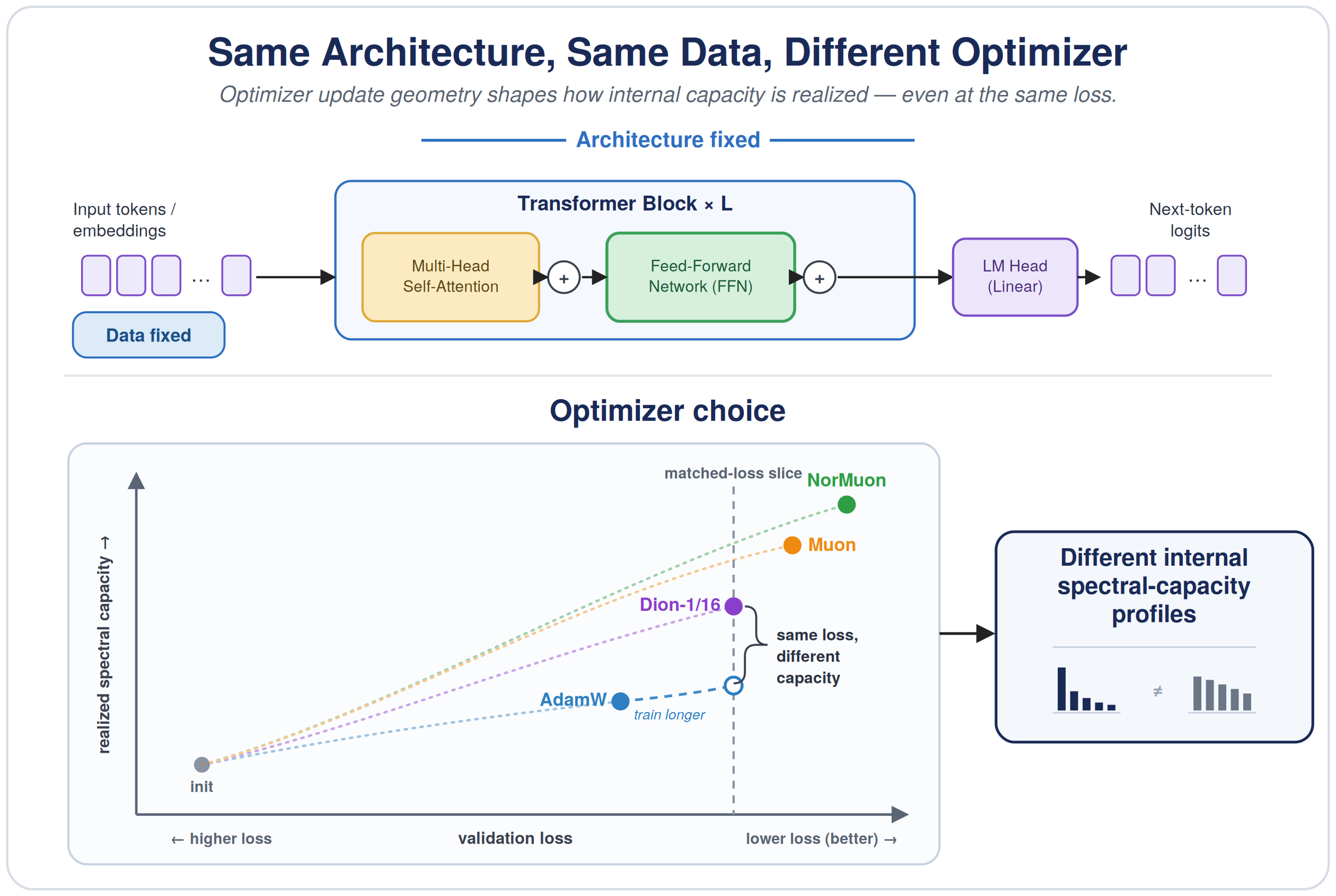
- Finding. Holding architecture, training data, tokenizer, and FFN-width schedule fixed, optimizer choice changes the spectral capacity realized inside FFN representations.
- Matched loss is not matched representation. The same architecture can reach similar validation loss under different optimizers while learning different representations. Longer AdamW training can match Dion-1/16 (a distributed low-rank-update optimizer; Ahn et al., 2025) in validation loss, but not in capacity scaling: extending training improves loss while the hard-rank scaling exponent drops from 0.29 to 0.03.
- Implication. Architecture determines the available degrees of freedom, training dynamics determine which of them become active, variance-carrying representation directions, and how they are allocated across token-frequency regimes. The effect is strongest for rare tokens, where sparse supervision leaves more room for optimizer-induced bias to shape the learned representation.
Throughout this post, realized capacity means realized spectral capacity: variance-carrying eigenmodes in FFN eigenspectrum representation. Note that it is not a complete measure of intelligence, transfer, or downstream capability; it is an internal telemetry signal that loss curves and parameter counts do not directly capture.
This post starts from a single finding and asks what follows from it. Classical scaling laws taught us to ask how loss changes with parameters, training data, and compute. They leave another question open: when we add architectural capacity, does training convert it into useful internal structure? In our experiments, that conversion depends strongly on optimizer choice, especially in rare-token regimes where supervision is sparse.
On this page
1. Same architecture, different capacity scaling
When architecture, training data, tokenizer, and FFN-width schedule are fixed, changing the optimizer changes how realized spectral capacity scales.
Four quantities help interpret the result.
- Diffuse capacity: soft spectral rank, how broadly representation variance spreads across eigenmodes.
- Dominant-mode capacity: hard spectral rank, how many eigenmodes carry substantial variance.
- Capacity asymmetry: the gap between soft and hard rank. It diagnoses whether capacity is broadly distributed across many eigenmodes or concentrated in a few dominant directions. Lower asymmetry means a more even spread.
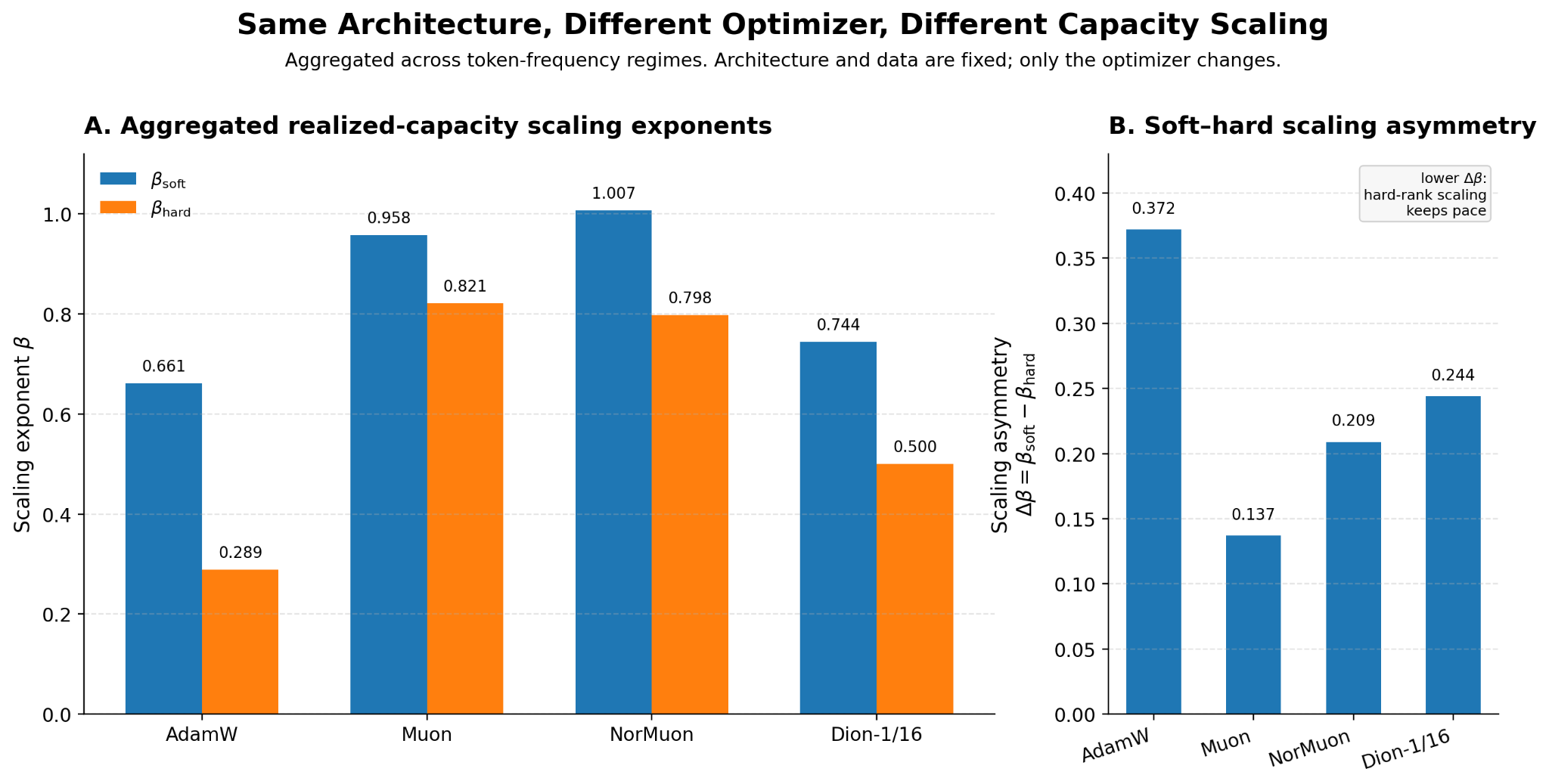
- Scaling exponent: how quickly realized capacity grows as FFN width increases.
We vary FFN width within the same model family and compare how realized spectral capacity grows. The model does not merely train faster or slower; it converts the same architectural budget into a different internal-capacity profile.
Figure 1 gives the global view of realized capacity scaling. AdamW shows the weakest dominant-mode scaling ($\beta_{\mathrm{hard}} \approx 0.29$), while Muon and NorMuon achieve near-linear scaling ($\beta_{\mathrm{hard}} \approx 0.80$), roughly a $2.8\times$ larger exponent under the same architecture and training data. This gap becomes more pronounced in the rare-token regime, which Section 3 examines.
The full result tables, frequency-conditioned fits, and ablations are on the project page.
These are GPT-2-scale studies, including 160M and 350M model families on FineWeb-Edu. They show that optimizer choice can change realized spectral capacity scaling under matched architecture and training data; they do not guarantee that the same optimizer ordering must persist at multi-billion-parameter scale. Establishing this would require a calibrated billion-scale sweep that holds architecture, training data, tokenizer, and FFN-width schedule fixed while measuring whether the same diffuse, dominant-mode, and HEAD/MID/TAIL effects persist.
Takeaway. Optimizer choice can change not only convergence speed or final loss, but the scaling law exponents by which added FFN width becomes realized spectral capacity.
2. Matched loss is not matched representation
A natural objection is that one optimizer may merely train faster. The matched-loss comparison tests that possibility.
Extending AdamW training from 6K to 12K training steps improves validation perplexity and brings it close to Dion-1/16 across the FFN-width sweep. But the realized-capacity scaling does not match; AdamW-12K remains much weaker in dominant-mode capacity scaling.
The scaling trend is counterintuitive: longer AdamW training improves loss but weakens dominant-mode scaling—the hard-rank exponent drops from 0.29 to 0.03. That is, the added FFN width no longer converts into spectral capacity, particularly in wider models, even when loss continues to improve.
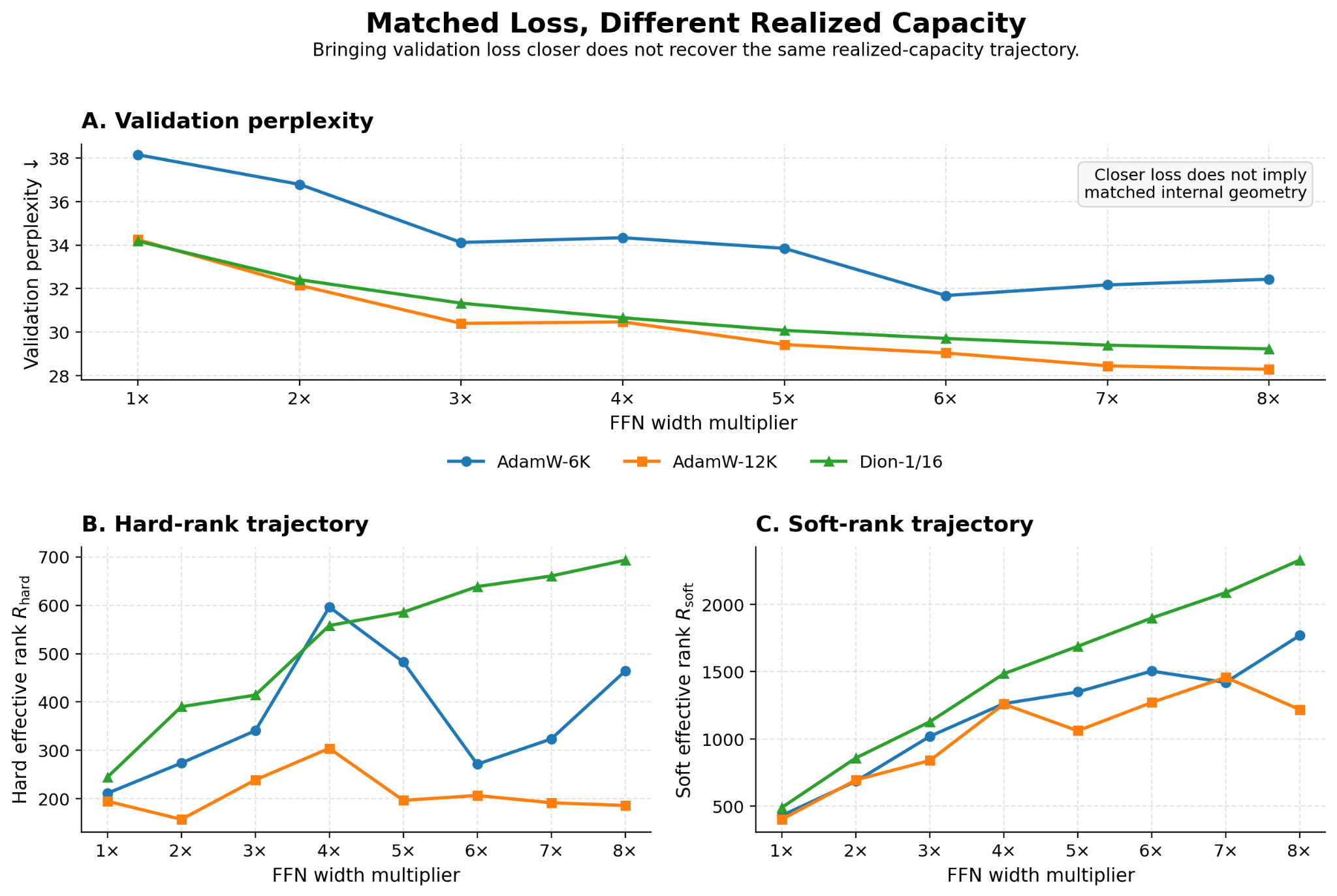
This gap is not an artifact of learning-rate tuning. Our learning-rate sweep shows that the spectral gap persists across learning rates. Practically, two training runs can look similar by loss while realizing very different internal capacity. Loss measures average output error; it does not establish that training produced the same representation directions, solution geometry, or adaptation-relevant internal structure.
Takeaway. Matched validation loss can still mask different width-to-capacity realization trajectories. Loss matching is necessary for a fair comparison, but it is not enough to establish matched representation geometry.
3. Rare tokens expose optimizer-induced capacity allocation
Natural language is long-tailed, and language models are known to struggle disproportionately on its rare tokens (Kandpal et al., 2023). A small number of HEAD tokens receive dense, repeated training signal; TAIL tokens receive sparse, noisy, intermittent signal.
This suggests a straightforward regime-dependent interpretation. For HEAD tokens, dense supervision leaves optimizers less room to produce qualitatively different representations. For TAIL tokens, sparse supervision gives optimizer-induced bias more degrees of freedom in determining which weak signals become variance-carrying representation directions.
In Bayesian terms, dense regimes are likelihood-dominated, while sparse regimes are more prior-sensitive. In this analogy, the optimizer contributes an implicit bias over which solutions training is likely to reach. This makes the TAIL a particularly important place to look for optimizer-induced differences in capacity allocation.
| Token regime | How constrained by data? | Key spectral observations | Design focus |
|---|---|---|---|
| HEAD | Strong | Optimizer gap is smallest; architecture is most competitive in hard-rank scaling | Architecture-sensitive |
| MID | Partial | Optimizer gap widens; Muon/NorMuon reduce soft–hard asymmetry relative to AdamW | Architecture–optimizer co-design |
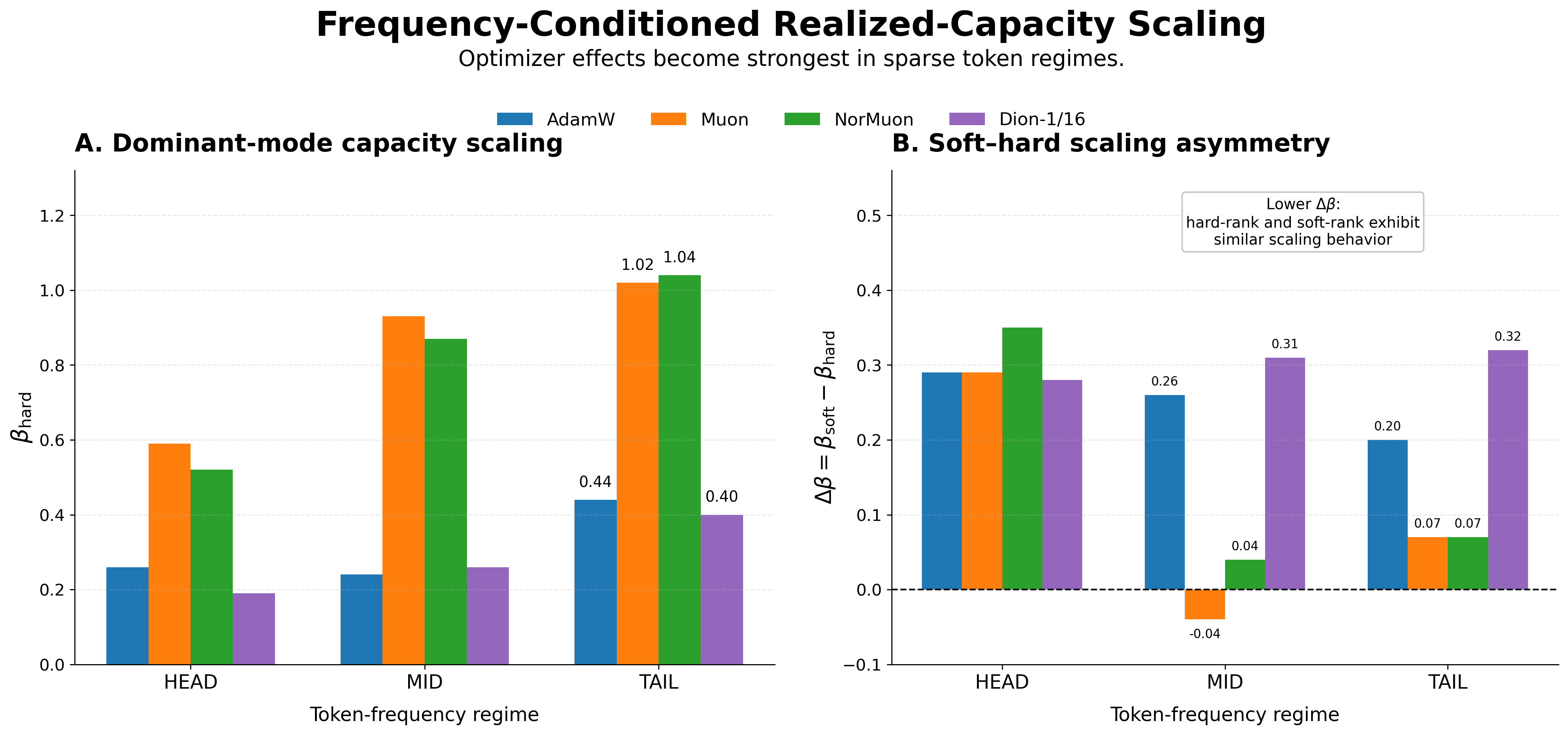
| TAIL | Weak | Optimizer choice dominates hard-rank scaling ($\beta_{\mathrm{hard}} \approx 0.44$ vs $\approx 1.0$) | Optimizer and training dynamics |
All three regimes are measured directly in Figure 3, so the table summarizes observed spectral behavior rather than extrapolating from a single regime. Token frequency is a proxy for how strongly the data constrains a token’s representation. The optimizer effect is present across the distribution, but grows as that constraint weakens — smallest in HEAD, larger in MID, and strongest in TAIL. The last column should be read narrowly: HEAD is not “architecture-only”; rather, in these hard-rank measurements, architectural changes are most competitive in the HEAD regime.
This is why architecture-only changes can under-deliver for long-tail behavior: adding capacity raises the nominal ceiling, but sparse training signal does not automatically convert that capacity into variance-carrying directions. The optimizer may need to preserve and amplify weak signals rather than let them vanish or fragment.
This makes the result relevant to capability-oriented pretraining questions. If realized capacity affects transfer in sparse regimes, then low-resource languages, rare scientific and code vocabulary, long-tail factual recall, tool-use edge cases, and sparse expert specialization are natural places to test this diagnostic. Spectral measurement alone does not prove that behavioral connection.
Figure 3 resolves the aggregate result from Figure 1 into HEAD, MID, and TAIL regimes. The left panel shows dominant-mode scaling through $\beta_{\mathrm{hard}}$. In TAIL representations, AdamW and Dion-1/16 have substantially weaker hard-rank scaling, with AdamW at $\beta_{\mathrm{hard}} \approx 0.44$, while Muon and NorMuon approach near-linear dominant-mode growth, $\beta_{\mathrm{hard}} \approx 1.0$—roughly a $2.3\times$ larger exponent. For Dion-1/16, spectral scaling behavior remains closer to AdamW than to Muon/NorMuon in the TAIL regime. The right panel shows the scaling asymmetry, $\Delta\beta = \beta_{\mathrm{soft}} - \beta_{\mathrm{hard}}$: Muon and NorMuon keep soft- and hard-rank scaling nearly aligned, while AdamW shows a larger gap.
Since loss is an aggregate metric, it can be dominated by frequent tokens and obscure whether rare tokens receive realized spectral capacity. A capacity-aware training run should therefore ask not only whether average loss improved, but whether the long tail received measurable internal structure that predicts rare-regime behavior.
Takeaway. Rare-token regimes are where optimizer-induced bias most strongly shapes which weak signals become variance-carrying representation directions.
4. Three views of the same gap
The result is not merely an optimizer-specific observation. It points to a broader gap: scalar objective value, nominal architecture, and learned internal representation are often conflated, but they are not the same object.
Section 2 made this concrete: matched validation loss can mask different spectral-capacity trajectories. The three views below generalize it for pretraining science.
| View | Main lesson | What it adds here |
|---|---|---|
| Scalar objectives under-identify internal structure | Similar loss can mask different learned representations. | Places the matched-loss result inside a broader failure mode of loss-only comparison. |
| Nominal capacity is not realized capacity | Width matters only if training converts it into variance-carrying representation directions. | Names the missing internal axis: how much architectural capacity becomes realized spectral capacity. |
| Reachable solution is optimizer-conditional | The same architecture does not imply the same reachable solution. | Explains why optimizer-induced bias can shape capacity allocation, even under fixed architecture. |
The sequence moves from measurement to mechanism: scalar objectives can obscure the model’s internal state, realized capacity names the missing internal axis, and optimizer-induced bias explains why the reachable solution can change under fixed architecture.
View I — Scalar objectives under-identify internal structure
Loss, gradient norms, and downstream evaluations are useful signals, but no single scalar metric fully describes a trained model’s learned representation or solution geometry. The same value can arise from different internal structures: variance may spread across many directions, concentrate in a few dominant modes, or appear unevenly across token-frequency regimes. The matched-loss result above is one spectral-capacity instance of this broader under-identification problem.
The upstream–downstream literature gives empirical precedent. The same pretraining loss can still produce different downstream transfer (Liu et al., 2022), different geometry among task-specific minima (Chen et al., 2026), and non-monotonic changes in learned representation geometry that scalar metrics miss (Li et al., 2025a). Theoretical work makes the same point: low pretraining loss alone need not guarantee that every downstream-relevant feature is recoverable from the representation (Wu, Lee, and Ge, 2023). In this post, realized spectral capacity provides one measurable axis of that under-identification.
Rate–distortion theory gives a useful formal analogy. A scalar objective can identify one point on a trade-off surface without specifying the internal allocation that produced it. Alemi et al., 2018 show that fixing the ELBO corresponds to a point on a rate–distortion curve, so models with the same ELBO can occupy different rate–distortion tradeoffs; changing the objective weights moves the solution along that curve. Gao and Chaudhari, 2020 generalize this to an equilibrium surface relating rate, distortion, and loss, where different multipliers can reach different internal tradeoffs at the same loss.
Our setting has the same structural shape, but not the same literal variables. Validation loss is the scalar coordinate; realized spectral capacity is one internal allocation it leaves underdetermined; and optimizer choice plays a role analogous to a multiplier, selecting which region of training geometry is reached. Spectral rank is not rate, and we impose no explicit rate–distortion objective.
The question is therefore not only how low did loss go? but also:
What internal capacity did training realize in order to reach that loss?
View II — Nominal capacity is not realized capacity
The architecture–optimizer distinction becomes clearest if we separate two notions of capacity.
Nominal capacity is the capacity implied by the architecture: parameter count, width, depth, heads, experts, routing paths, memory layout, and FLOPs.
Realized spectral capacity is the capacity measured as active variance-carrying structure inside the trained model: which representation directions become active, how variance is distributed across eigenmodes, which modes grow with width.
Architecture gives the learning system things optimization cannot create: causal masking, equivariance, sparse routing, dimensional ceilings, and residual topology. But architecture creates nominal capacity — the available degrees of freedom — and does not guarantee that training will use all of them.
A useful mental model is:
Here, $\mathcal{A}$ is the architecture, $\mathcal{O}$ is the optimizer/training algorithm, and $\mathcal{D}$ is the training data. This is not a literal scalar law; it is a design principle. Architecture sets nominal capacity. Optimization and training data influence how much of that capacity is realized in representation space. Whether that structure is behaviorally useful must be tested separately.
The same architectural intervention can therefore have different realized effects under different optimizers. If $\rho_{\mathrm{realized}}$ is high, added width translates into measured representation capacity. If it is low, added width raises the ceiling without filling it.
To measure this distinction, we look at spectral geometry. Given a representation covariance, its eigenspectrum characterizes how variance is distributed across eigenmodes. Effective-rank measures summarize that distribution; the entropy-based formulation traces back to Roy and Vetterli, 2007, and the Rényi family varies sensitivity to diffuse versus dominant eigenmodes (Rényi, 1961).
Let the eigenvalues of a representation covariance be $(\lambda_1, \ldots, \lambda_d)$, and normalize them into a variance distribution over eigenmodes:
For this post, two effective ranks are enough:
These are the two capacity measures from Section 1, now made precise: diffuse capacity is the soft spectral rank, $R_{\mathrm{soft}} = R_1$; dominant-mode capacity is the hard spectral rank, $R_{\mathrm{hard}} = R_2$. Capacity asymmetry is their log-ratio, $\log\left(R_{\mathrm{soft}} / R_{\mathrm{hard}}\right)$, the multiplicative gap between diffuse and dominant-mode capacity in a single model.
Because $R_{\mathrm{soft}}$ and $R_{\mathrm{hard}}$ are Rényi effective ranks of orders 1 and 2, and Rényi rank is non-increasing in the order, the hard rank can never exceed the soft rank. This makes the upper-left region of the phase map in Figure 4 necessarily forbidden, not merely unobserved, and the frontier $R_{\mathrm{hard}} = R_{\mathrm{soft}}$ a true boundary. The exponent gap reported in the figures, $\Delta\beta = \beta_{\mathrm{soft}} - \beta_{\mathrm{hard}}$, measures how capacity asymmetry scales as the FFN widens.
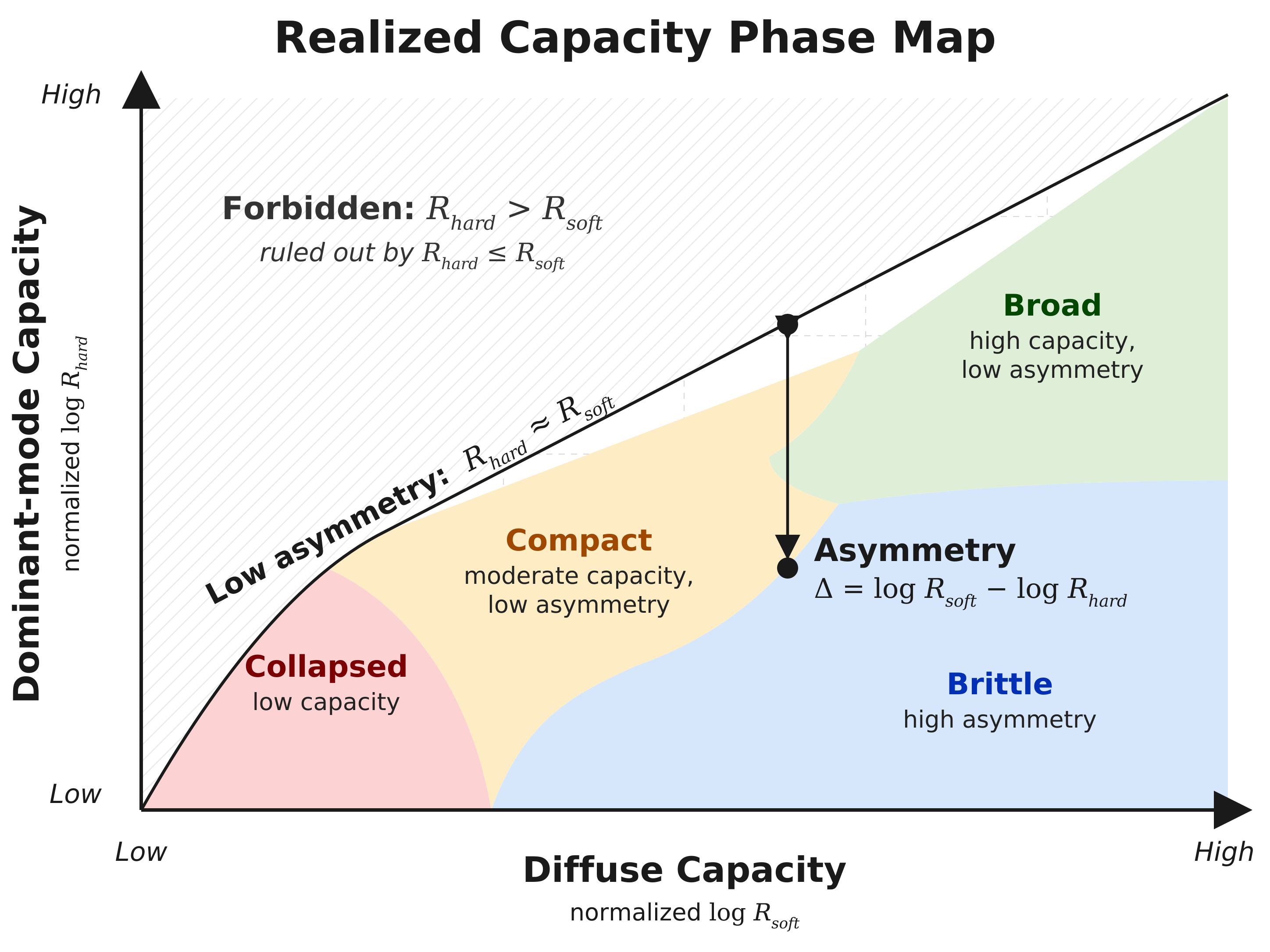
This phase map separates realized-capacity profiles that a single loss value can conflate: collapsed, with low capacity; compact, with moderate capacity and low asymmetry; broad, with high capacity and low asymmetry; and brittle, with high asymmetry. Capacity asymmetry measures whether broad spectral spread is matched by substantial variance in dominant eigenmodes. This is what separates brittle profiles from compact and broad ones.
View III — Reachable solution is optimizer-conditional
Realized capacity can differ under the same architecture because learning is shaped by more than structural design. Training data rarely specifies a unique solution; it leaves many data-consistent models possible, and inductive biases decide which ones are favored (Goldblum et al., 2024).
Architecture supplies structural biases; causal masking, residual topology, attention structure, parameter sharing, routing, width, and depth constrain which computations are available. The optimizer supplies dynamical biases; it does not change the formal architecture, but it changes the trajectory through parameter space — which solutions are reachable, stable, and likely under a fixed training budget. This is consistent with the view that overparameterized learning preserves a broad hypothesis space while imposing softer preferences over data-consistent solutions (Wilson, 2025).
What this post adds is a way to measure one such dynamical preference. Realized spectral capacity tracks which representation directions training turns into variance-carrying structure, giving a concrete axis along which optimizers can differ even when their loss curves look similar.
Forward-looking implication: realized capacity may matter for plasticity
Continual learning raises a forward-looking version of the same question. Forgetting asks whether a model retains the past; plasticity asks whether it can still learn the future. This is a conjectural extension of the spectral measurements in this post: we measure realized capacity at a fixed point, whereas future learnability depends on whether enough representation directions remain available for later adaptation.
The reason the conjecture matters is that loss can decouple from adaptability, just as it decouples from realized capacity. Han et al., 2026 showed that larger (pre-)training weight decay yields more adaptable base models — larger downstream gains after fine-tuning — even though those base models reach higher pretraining loss. That is, the most adaptable base model is not necessarily the one with the lowest pretraining loss, and accepting a worse pretraining loss can buy better adaptation to later tasks. Similar observations are reported by Hernandez-Garcia et al., 2026; GPT-style LLMs trained on long multilingual streams lose the ability to efficiently learn a held-out language as training continues.
If a model’s future ability to learn depends on how many representation directions remain active, then realized capacity becomes a natural plasticity diagnostic. A consistent observation made in the plasticity literature is the loss of active directions; dormant units, falling effective feature rank, or degenerating curvature spectra across reinforcement learning, vision, and language (Abbas et al., 2023; Dohare et al., 2024; Lyle et al., 2024; He et al., 2025).
Two complementary biases on one quantity. Realized capacity tracks the representation directions that become active and variance-carrying. Architecture supplies the structural constraints; optimization supplies the dynamical bias that determines which of those directions are actually realized during training.
| Architecture — structural bias | Optimizer — dynamical bias | |
|---|---|---|
| Role | Creates capacity by constraining which directions can carry signal | Realizes capacity by shaping which directions actually do carry signal |
| When it acts | Chosen at design time; constrains the training trajectory throughout | Acts throughout training; tunable via optimizer choice, schedule, and regularization |
| How capacity is lost | Rank bottlenecks, poor width/depth balance, unstable or collapsing pathways | Dormant units, gradient singular-value collapse, norm growth, optimizer-induced concentration |
| How capacity is preserved | Non-collapsing rank pathways, width/depth balance, architecture-level plasticity mechanisms | Orthogonalized updates, weight decay, targeted resets, and optimizer choices that keep spectra balanced |
On the architectural side, width and depth appear to shape different parts of the plasticity trade-off: wider networks tend to forget less, while deeper networks remain more plastic (Mirzadeh et al., 2022; Lu et al., 2025). Architectural interventions such as interpolation layers can also maintain a non-collapsing rank contribution without changing the optimizer (Koeppe et al., 2026).
On the optimizer side, plasticity can be restored by adding a fraction of the gradient’s polar factor to each update, raising near-zero singular values that stability-preserving methods otherwise drive toward collapse (Zheng et al., 2026). Notably, this polar factor is mathematically related to the orthogonalization operation used in Muon-style updates. This makes the connection suggestive: the same class of geometry-shaping updates that changes spectral capacity here may also help preserve plasticity.
At LLM scale, additional parameters postpone the onset of plasticity loss, but only sublinearly — delaying collapse without preventing it (Hernandez-Garcia et al., 2026) — while larger models can retain rare-task structure longer by reducing gradient interference between tasks (Huang et al., 2026).
The continual-learning implication is not that architecture ceases to matter. It is that capacity must be both realized during pretraining and preserved in a form that remains available for later learning. This is close to what formal definitions of plasticity try to measure; how much an agent can still be shaped by what it observes (Abel et al., 2025). Which directions remain available depends jointly on architecture, optimizer, regularization, and training dynamics.
5. Why optimizer choice changes capacity, not just speed
Views I–III showed that optimizer choice changes realized capacity, but they did not explain why an optimizer should affect representation geometry rather than merely convergence speed. The key point is that an optimizer defines an update geometry: it transforms raw gradients into parameter updates through coordinate-wise scaling, weight decay, momentum, matrix preconditioning, orthogonalization, or constrained update subspaces. These choices can change which representation directions grow, which eigendirections accumulate variance, and which weak signals persist long enough to become coherent representation structure.
| Mechanism | Examples | How it can affect realized capacity |
|---|---|---|
| Adaptive scaling and weight decay | AdamW-style updates (Loshchilov and Hutter, 2019) | Change per-parameter update scale, norm growth, and which same-loss solutions are easier to reach |
| Matrix or tensor preconditioning | Shampoo-style structure-aware updates (Gupta, Koren, and Singer, 2018) | Change the conditioning of weight updates and how added width becomes active representation structure |
| Matrix orthogonalization | Muon and NorMuon-style updates (Jordan et al., 2024; Liu et al., 2025; Li et al., 2025b) | Change update geometry across weight matrices, altering which eigendirections accumulate substantial variance |
| Low-rank or communication-constrained updates | Dion-style updates (Ahn et al., 2025) | Restrict the update subspace and reshape how capacity is allocated across modes and token regimes |
The claim is not that one optimizer mechanism is universally better. It is that each optimizer defines a different training geometry. These choices do not change the formal architecture, but they change the trajectory through parameter space: which solutions are reachable, which update directions are amplified, which weak signals survive, and which representation eigendirections become variance-carrying structure. This makes matched loss an incomplete description of what the model has learned internally. Optimizer choice therefore belongs inside the capacity-scaling object, not merely in the training recipe.
In practice, scaling decisions should specify both architecture and optimizer, and optimizer comparisons should report not only speed and loss but also the quality of the representation they induce. This raises a pretraining question: what should we log to know whether added architectural capacity became realized internal structure?
6. What changes in pretraining practice?
Loss remains the central training objective and a low-variance signal for scaling laws; nothing here proposes replacing it. What loss alone does not reveal is the kind of solution the model is converging toward: whether it is using its parameter budget effectively, where capacity appears across the data distribution, or whether a given architecture–optimizer pair induces the desired representation geometry. For that, we need internal telemetry.
A capacity-aware pretraining report should answer five practical questions:
| Question | Diagnostic | What it catches |
|---|---|---|
| Did same-loss models build the same representation? | Matched-loss optimizer comparisons | Similar perplexity masking different representation geometry |
| Does added FFN width become realized capacity? | Diffuse and dominant-mode capacity scaling | Wider models whose dominant modes do not grow |
| Is capacity broadly spread but weakly concentrated? | Capacity asymmetry | Diffuse capacity growing without matched dominant-mode structure |
| Where in the data distribution does capacity appear? | Frequency-conditioned capacity across HEAD, MID, and TAIL regimes | Average loss improving while long-tail regimes remain under-realized |
| Is the effect tied to a design pair? | Architecture–optimizer interaction sweeps | Attributing to architecture alone what depends on the optimizer |
These diagnostics are lightweight telemetry signals. They make optimizer comparisons more informative: not only which optimizer reaches a target loss fastest, but how each one realizes the same architecture’s capacity.
The same measurements extend beyond a single training run. Classical scaling laws predict loss from parameters, data, and compute (Kaplan et al., 2020; Hoffmann et al., 2022) and remain central. A capacity-aware scaling law would complement them with internal variables — diffuse capacity, dominant-mode capacity, capacity asymmetry, and frequency-conditioned capacity — as functions of width, depth, optimizer, and data. This also aligns with recent arguments that AI systems should be studied as training processes, not only as static artifacts analyzed after training (Biderman et al., 2026).
Logging this telemetry is inexpensive. Soft and hard ranks are computed from the eigenspectrum of a layer’s FFN post-activation covariance, requiring eigenvalues but not stored eigenvectors. In our prior ICLR 2026 work, logging these quantities every 1,000 steps on GPT-2-scale runs added roughly 1% wall-clock overhead and tens of megabytes of GPU memory.
The logging strategy should distinguish monitoring from final measurement. Pre-activation spectra are stable under token subsampling and are useful for low-cost, frequent monitoring. Post-activation spectra are more sensitive, especially hard-rank estimates in the tail, because the nonlinearity and token sparsity make the mid-to-tail eigenspectrum easier to distort. A practical strategy is therefore two-level; use pre-activation soft and hard ranks for frequent telemetry, and use full-batch post-activation ranks when making claims about realized capacity.
7. What this does not claim
The claim here is specific and empirical: when architecture, training data, and tokenizer are held fixed, optimizer choice can change realized spectral capacity. The following points clarify what this result does not establish.
First, spectral rank is not a complete theory of intelligence, generalization, or downstream ability. It is a principled measure of representational structure and should be read alongside held-out loss, task-level performance, controlled ablations, and other problem-specific measures.
Second, higher realized spectral capacity is not automatically better in every setting. The important question is not simply whether capacity increases, but where that capacity appears, whether it is stable, and whether it predicts behavior, transfer, or future learnability.
Third, optimizer–architecture co-design does not imply that the optimizer replaces architecture. Architecture remains a fundamental constraint: optimizers cannot create what the architecture does not support, or remove inference costs imposed by the computation graph. They also cannot represent functions outside the model hypothesis class.
Fourth, the scale question remains open. The evidence here shows that optimizer choice changes realized spectral capacity at the GPT-2 160M/350M scale. Stronger claims require larger models, longer training runs, broader architectural families, downstream performance analysis, continual-learning tests, and direct studies of rare-regime behavior.
8. Open questions
If realized capacity is measurable and optimizer-conditional, the open research questions become concrete: what it predicts and reveals about internal computation, how architecture and optimization interact, and how these measurements should complement loss-based scaling laws in guiding model design.
1. Which spectral differences predict downstream behavior? If two models have similar loss but different realized capacity, which spectral axes predict transfer, robustness, rare-token reliability, or domain adaptation?
2. Does realized capacity predict plasticity and future learnability? A model with similar loss but different spectral allocation may differ in its ability to keep learning. Capacity telemetry may therefore help diagnose loss of plasticity, representational collapse, or exhaustion of useful directions during continued training.
3. Are effective computational graphs optimizer-conditional? If the optimizer changes which routes through the model carry meaningful signal, then circuits discovered in one trained model may not be stable across optimizers, even with the same architecture (Elhage et al., 2021).
4. How do architecture and optimizer modulate each other? Architectural interventions do not act in isolation; their effects are modulated by the optimizer. Removing RoPE, for example, changes perplexity by different amounts across optimizers. A similar interaction appears inside the FFN: the nonlinearity can reorder realized-capacity differences across optimizers, so the optimizer with the highest pre-activation capacity is not necessarily the one with the highest post-activation capacity. The open question is whether such interactions can be predicted from the architecture–optimizer pair.
5. How should we search over architecture–optimizer pairs? Neural architecture search typically fixes the optimizer. Optimizer evaluation typically fixes the architecture. The co-design view suggests that this may miss regions where neither component looks optimal alone, yet their correct pairing offers stronger performance.
9. Conclusion: toward capacity-aware LLM design
The key finding is: if two optimizers train the same architecture but produce different spectral-capacity scaling, optimizer choice has changed the model’s realized capacity. The matched-loss comparison in Figure 2 strengthens this point: similar validation loss does not imply matched representation geometry. Further, Figure 3 shows where the measured difference is largest: MID and TAIL regimes, where optimizer-induced bias can shape capacity allocation across the data distribution.
The three views above point to the same gap: scalar objectives are not internal structure, nominal capacity is not realized capacity, and reachable capacity is optimizer-conditional.
The next generation of model design should therefore ask more than how many parameters we train, how many tokens we consume, or how low the loss goes. It should also ask what capacity becomes realized and where it appears in the data distribution.
Capacity-aware LLM design means tracking not only what the model could represent, but what training actually realized — and then testing which realized directions support behavior, transfer, and future learning.
Citation
If you find this post useful, please cite the associated paper.
@article{jha2026optimizerinduced,
  title   = {Same Architecture, Different Capacity: Optimizer-Induced Spectral Scaling Laws},
  author  = {Jha, Nandan Kumar and Reagen, Brandon},
  year    = {2026},
  url     = {https://arxiv.org/abs/2605.21803}
}
References
Scaling laws
- Kaplan, J., McCandlish, S., Henighan, T., Brown, T. B., Chess, B., Child, R., Gray, S., Radford, A., Wu, J., and Amodei, D. Scaling Laws for Neural Language Models. arXiv:2001.08361, 2020. arXiv
- Hoffmann, J. et al. Training Compute-Optimal Large Language Models. NeurIPS, 2022. arXiv
Upstream–downstream behavior
- Liu, H., Xie, S. M., Li, Z., and Ma, T. Same Pre-training Loss, Better Downstream: Implicit Bias Matters for Language Models. arXiv:2210.14199, 2022. arXiv
- Wu, J., Lee, J. D., and Ge, R. Connecting Pre-trained Language Models and Downstream Tasks via Properties of Representations. NeurIPS, 2023. NeurIPS
- Chen, H., Zhang, H., Li, X., Dong, Y., Shen, K., and Zhu, J. Nexus: Same Pretraining Loss, Better Downstream Generalization via Common Minima. arXiv:2604.09258, 2026. arXiv
- Li, M. Z., Agrawal, K. K., Ghosh, A., Teru, K. K., Santoro, A., Lajoie, G., and Richards, B. A. Tracing the Representation Geometry of Language Models from Pretraining to Post-training. arXiv:2509.23024, 2025a. arXiv
- Biderman, S., Khan, M. A., Mireshghallah, N., Arnett, C., Barez, F., and Saphra, N. Position: Don't Just "Fix it in Post": A Science of AI Must Study Training Dynamics. arXiv:2606.06533, 2026. arXiv
- Kandpal, N., Deng, H., Roberts, A., Wallace, E., and Raffel, C. Large Language Models Struggle to Learn Long-Tail Knowledge. ICML, 2023. arXiv
Optimization and optimizer-induced bias
- Loshchilov, I., and Hutter, F. Decoupled Weight Decay Regularization. ICLR, 2019. arXiv
- Gupta, V., Koren, T., and Singer, Y. Shampoo: Preconditioned Stochastic Tensor Optimization. ICML, 2018. arXiv
- Jordan, K. et al. Muon: An Optimizer for Hidden Layers in Neural Networks. Original public technical write-up, 2024. write-up
- Liu, J. et al. Muon is Scalable for LLM Training. arXiv:2502.16982, 2025. arXiv
- Li, Z., Liu, L., Liang, C., Chen, W., and Zhao, T. NorMuon: Making Muon More Efficient and Scalable. arXiv:2510.05491, 2025b. arXiv
- Ahn, K., Xu, B., Abreu, N., and Langford, J. Dion: Distributed Orthonormalized Updates. arXiv:2504.05295, 2025. arXiv
Spectral capacity and information-theoretic framing
- Alemi, A. A., Poole, B., Fischer, I., Dillon, J. V., Saurous, R. A., and Murphy, K. Fixing a Broken ELBO. ICML, 2018. PMLR
- Gao, Y., and Chaudhari, P. A Free-Energy Principle for Representation Learning. ICML, 2020. PMLR
- Rényi, A. On Measures of Entropy and Information. Proceedings of the Fourth Berkeley Symposium on Mathematical Statistics and Probability, 1961. Project Euclid
- Roy, O., and Vetterli, M. The Effective Rank: A Measure of Effective Dimensionality. EUSIPCO, 2007. PDF
- Jha, N. K., and Reagen, B. NerVE: Nonlinear Eigenspectrum Dynamics in LLM Feed-Forward Networks. ICLR, 2026. arXiv
Inductive bias and interpretability
- Goldblum, M., Finzi, M., Rowan, K., and Wilson, A. G. The No Free Lunch Theorem, Kolmogorov Complexity, and the Role of Inductive Biases in Machine Learning. ICML, 2024. arXiv
- Wilson, A. G. Deep Learning is Not So Mysterious or Different. ICML, 2025. arXiv
- Elhage, N. et al. A Mathematical Framework for Transformer Circuits. Transformer Circuits, 2021. article
Plasticity and continual learning
- Mirzadeh, S. I., Chaudhry, A., Yin, D., Hu, H., Pascanu, R., Gorur, D., and Farajtabar, M. Wide Neural Networks Forget Less Catastrophically. ICML, 2022. arXiv
- Lu, A., Yuan, H., Feng, T., and Sun, Y. Rethinking the Stability-Plasticity Trade-off in Continual Learning from an Architectural Perspective. ICML, 2025. arXiv
- Abbas, Z., Zhao, R., Modayil, J., White, A., and Machado, M. C. Loss of Plasticity in Continual Deep Reinforcement Learning. arXiv:2303.07507, 2023. arXiv
- Dohare, S., Hernandez-Garcia, J. F., Lan, Q., Rahman, P., Mahmood, A. R., and Sutton, R. S. Loss of Plasticity in Deep Continual Learning. Nature, 2024. article
- Lyle, C., Zheng, Z., Khetarpal, K., van Hasselt, H., Pascanu, R., Martens, J., and Dabney, W. Disentangling the Causes of Plasticity Loss in Neural Networks. arXiv:2402.18762, 2024. arXiv
- He, N., Guo, K., Prakash, A., Tiwari, S., Tao, R. Y., Serapio, T., Greenwald, A., and Konidaris, G. Spectral Collapse Drives Loss of Plasticity in Deep Continual Learning. arXiv:2509.22335, 2025. arXiv
- Han, T., Bordt, S., Zhang, H., and Kakade, S. Weight Decay Improves Language Model Plasticity. ICML, 2026. arXiv
- Huang, J., Wurgaft, D., Bansal, R., Ruis, L., Saphra, N., Alvarez-Melis, D., Lampinen, A. K., Potts, C., and Lubana, E. S. Why Larger Models Learn More: Effects of Capacity, Interference, and Rare-Task Retention. arXiv:2605.29548, 2026. arXiv
- Abel, D. et al. Plasticity as the Mirror of Empowerment. arXiv:2505.10361, 2025. arXiv
- Hernandez-Garcia, J. F., Figliolia, T., and Millidge, B. Can Scale Save Us From Plasticity Loss in Large Language Models? arXiv:2606.24752, 2026. arXiv
- Zheng, G., Yang, E., Wang, X., Chen, Y., He, F., Zheng, Q., Wang, P., and Shen, L. Plasticity Activation via Polar Operator: A Plug-in Method for Balancing Stability and Plasticity. ICML, 2026. OpenReview
- Koeppe, N., Vecchietti, L. F., Han, D., Li, D., and Lee, S. W. Mitigating Plasticity Loss through Architectural Design in Continual Learning. ICML, 2026. OpenReview